Interpretation

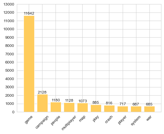
Viewing the top 10 game aspects tagged with a non-neutral sentiment polarity reveals that ‘game’ has by far the highest frequency.

Given the lack of specific information this aspect provides concerning specific design details, it will be useful to preclude this token from subsequent charts.

import matplotlib.pyplot as plt, seaborn as sns
df1=(df[df['sentiment']!=0]
     .groupby('aspect',as_index=False)['description']
     .count().rename(columns={'description':'Count'})
     .sort_values(by='Count',ascending=False)
     .head(10)).reset_index(drop=True)

sns.set_style('whitegrid')
p1=plt.bar(df1.aspect,df1.Count,align='center',color='#ffcc5c')
plt.xticks(rotation=45,ha='center')
plt.bar_label(p1,label_type='edge')
plt.yticks(list(range(0,13001,1000)));

Aspect Frequency

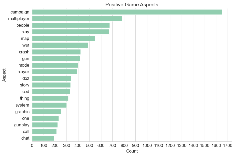
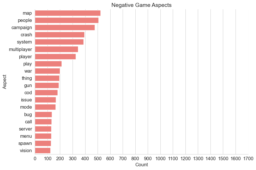
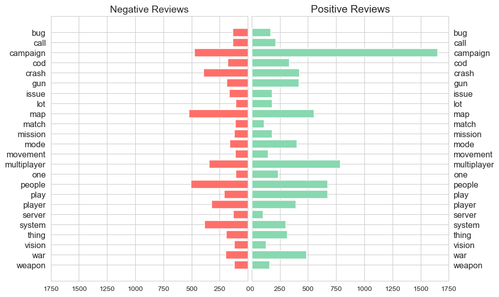
Charting the most frequent aspects tagged with a non-neutral score, it is clear how divisive many aspects of the game design are for the player base.

Several aspects feature in the top 20 of both sentiment lists which is indicative of the ‘mixed’ review score that game currently has on the Steam store.

While the campaign features promintently in both lists, the more than 1600 positive references far outstrip the number of negative references made in user reviews.

Similarly, the over 350 negative references to the game’s multiplayer aspect, is outweighed by almost 800 positive references.

The remainder of the overlapping aspects of design seem far more divisive and demonstrate more even splits in player opinion.

sns.set_style('whitegrid')
pos = (df[(df['sentiment']>0) & (df['aspect']!='game')]
                    .groupby('aspect')[['sentiment']]
                    .count().rename(columns={'sentiment':'Count'})
                    .sort_values(by='Count',ascending=False)
                    .reset_index()
                    .head(20))
                    
sns.catplot(data = pos,
            y='aspect',
            x='Count',
            kind='bar',
            palette = ['#88D8B0'],
            height = 6,
           aspect = 1.5)

plt.title('Positive Game Aspects',fontsize=14)
plt.tick_params(labelsize=12)
plt.ylabel('Aspect',fontsize=12)
plt.xlabel('Count',fontsize=12)
plt.xticks(list(range(0,1701,100)))
plt.tight_layout()
plt.show();

neg = (df[(df['sentiment']<0) & (df['aspect']!='game')]
                    .groupby('aspect')[['sentiment']]
                    .count().rename(columns={'sentiment':'Count'})
                    .sort_values(by='Count',ascending=False)
                    .reset_index()
                    .head(20))

sns.catplot(data = neg,
            y='aspect',
            x='Count',
            kind='bar',
            palette = ['#FF6F69'],
            height = 6,
           aspect = 1.5)
plt.title('Negative Game Aspects',fontsize=14)
plt.tick_params(labelsize=12)
plt.ylabel('Aspect',fontsize=12)
plt.xlabel('Count',fontsize=12)
plt.xticks(list(range(0,1701,100)))
plt.tight_layout()
plt.show();

Shared Aspects

neg1 = (df[(df['sentiment']<0) & (df['aspect']!='game')]
                    .groupby('aspect')[['sentiment']]
                    .count().rename(columns={'sentiment':'Count'})
                    .sort_values(by='Count',ascending=False)
                    .reset_index())
neg1 = neg1[neg1['Count']>99].set_index('aspect')

pos1 = (df[(df['sentiment']>0) & (df['aspect']!='game')]
                    .groupby('aspect')[['sentiment']]
                    .count().rename(columns={'sentiment':'Count'})
                    .sort_values(by='Count',ascending=False)
                    .reset_index())
pos1 = pos1[pos1['Count']>99].set_index('aspect')

pos1 = pos1.loc[pos1.index.intersection(neg1.index),].sort_index()
neg1 = neg1.loc[neg1.index.intersection(pos1.index),].sort_index()

graph, (plot1, plot2) = plt.subplots(1, 2,figsize=(10,6))
    
plot1.barh(neg1.index, neg1.Count, align='center',zorder=10,color = '#FF6F69')
plot1.set_xticks(list(range(0,1751,250)))
plot1.set_title('Negative Reviews',fontsize=14)
plot1.invert_xaxis()
plot1.invert_yaxis()
plot1.tick_params(axis='y',labelsize=12,right=False)

plot2.barh(neg1.index, pos1.Count, align='center',zorder=10,color = '#88D8B0')
plot2.set_xticks(list(range(0,1751,250)))
plot2.set_title('Positive Reviews',fontsize=15)
plot2.invert_yaxis()
plot2.yaxis.tick_right()
plot2.tick_params(axis='y',labelsize=12,right=False)

graph.tight_layout()
plt.subplots_adjust(wspace=0.02);

Aspect - Descriptor Links

The below plot visualises links between prominent aspects and descriptors.

To maintain plot legibility, aspects are restricted to the 20 highest frequency positve and 20 highest frequency negative aspects, descriptors are limited to those that appear 150 times or more in the corpus, and only links with a frequency greater than 25 are displayed.

The plot is interactive, aspect nodes can be selected to display associated links.

Here we can see that ‘campaign’ features many more links with several positive descriiptors (‘good’, ‘great’, ‘amazing’, ‘fun’) and comparitively fewer with the negative descriptor ‘bad’.

Likewise, ‘multiplayer’ displays more links with positive descriptors than negative.

import numpy as np
import holoviews as hv
from holoviews import opts, dim

hv.extension('bokeh')
hv.output(size=300)

# create list of aspects from top pos and neg lists
aspect_list = set(pos['aspect'].to_list() + neg['aspect'].to_list())

# Create df of top aspects across pos and neg sentiments
top_df = df[(df['aspect'].isin(aspect_list))]

# Create df of top descriptors across pos and neg sentiments
desc_counts = (top_df
     .groupby(by=['description'])[['sentiment']]
     .count()
     .rename(columns={'sentiment':'Count'})
     .sort_values(by ='Count', ascending =False)
     .reset_index())

# df containg top aspects and top descriptors
top_df = top_df = df[(df['aspect'].isin(aspect_list)) & (df['description'].isin(desc_counts[desc_counts['Count']>149]['description']))]

# quantify links
links = (top_df
     .groupby(by=['aspect','description'],as_index=False)[['sentiment']]
     .count()
     .rename(columns={'sentiment':'Count'}))
         
# specify node names
nodes = list(set(links['aspect'].tolist()))
nodes.extend(set(links['description'].tolist()))
nodes = hv.Dataset(pd.DataFrame(nodes, columns = ['Token']))

# efine function to rotate labels after 180
def rotate_label(plot, element):
    white_space = "              "
    angles = plot.handles['text_1_source'].data['angle']
    characters = np.array(plot.handles['text_1_source'].data['text'])
    plot.handles['text_1_source'].data['text'] = np.array([x + white_space if x in characters[np.where((angles < -1.5707963267949) | (angles > 1.5707963267949))] else x for x in plot.handles['text_1_source'].data['text']])
    plot.handles['text_1_source'].data['text'] = np.array([white_space + x if x in characters[np.where((angles > -1.5707963267949) | (angles < 1.5707963267949))] else x for x in plot.handles['text_1_source'].data['text']])
    angles[np.where((angles < -1.5707963267949) | (angles > 1.5707963267949))] += 3.1415926535898
    plot.handles['text_1_glyph'].text_align = "center"

# create chord diagram
chord = hv.Chord((links, nodes)).select(Count=(25, None))
chord.opts(
    opts.Chord(title='Reltionships Between Aspects and Descriptors', labels = 'Token', label_text_font_size='12pt', 
               node_color='Token', node_cmap=['#c1c1c1','#adadad'],node_size=10,
               edge_color='aspect', edge_cmap=['#FF6F69','#88D8B0','#ffcc5c'],
               hooks=[rotate_label], edge_alpha=0.8, edge_line_width=1)
)