Exploratory Data Analysis

PoS Tagging & Sentiment Scoring

The spaCy package [Honnibal et al., 2020] is used to assign part of speech tags to each token in the sample.

Subject nouns and associated adjectives are extracted and assigned as paired ‘aspect’ and ‘descriptor’.

The textblob package [Loria, 2021] is then applied to assign a sentiment polarity score to each:

Positive > 0.0
Neutral = 0.0
Negative < 0.0

import pandas as pd
df = pd.read_csv('data/preTag_df1.csv')

import spacy
nlp = spacy.load("en_core_web_sm")
from textblob import TextBlob

# split text into sentences and flatten
sentences = [str(x).split('.') for x in df.review_text]
sentences = [item for sublist in sentences for item in sublist]

# Extract aspects and descriptors
# Modified from https://towardsdatascience.com/aspect-based-sentiment-analysis-using-spacy-textblob-4c8de3e0d2b9
aspects = []
for sentence in sentences:
  doc = nlp(sentence)
  descriptors = ''
  target = ''
  for token in doc:
    if token.dep_ == 'nsubj' and token.pos_ == 'NOUN':
      target = token.text
    if token.pos_ == 'ADJ':
      prepend = ''
      for child in token.children:
        if child.pos_ != 'ADV':
          continue
        prepend += child.text + ' '
      descriptors = prepend + token.text
  aspects.append({'aspect': target,'description': descriptors})

# remove entries with blank aspect or descriptor
aspects = [x for x in aspects if x['aspect']!='' and x['description']!='']

# Add sentiment polarity scores
for aspect in aspects:
  aspect['sentiment'] = TextBlob(aspect['description']).sentiment.polarity

tag_df = pd.DataFrame(aspects)
display(tag_df.sort_values(by='sentiment',ascending=False).head(10).reset_index(drop=True))

	aspect	description	sentiment
0	game	awesome	1.0
1	duty	awesome	1.0
2	person	awesome	1.0
3	chat	so awesome	1.0
4	system	now perfect	1.0
5	game	awesome	1.0
6	ward	perfect	1.0
7	campaign	just superb	1.0
8	mode	awesome	1.0
9	game	perfect	1.0

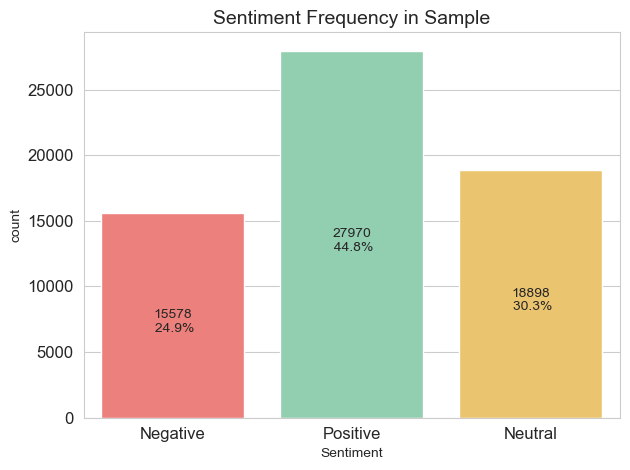
Sentiment Frequency

Graphing the frequency of each sentiment reveals that a large number (30.3%) of all aspects from the sample have been classified as neutral.

While this isn’t neccessarily out of the ordinary, some investigation of the neutral category may be worthwhile.

import numpy as np
tag_df['Sentiment'] = np.select([(tag_df['sentiment']>0),(tag_df['sentiment']<0),(tag_df['sentiment']==0)],['Positive','Negative','Neutral'])

import matplotlib.pyplot as plt
import seaborn as sns

sns.set_style('whitegrid')
ax=sns.countplot(data=tag_df,
              x="Sentiment", 
              palette = ['#FF6F69','#88D8B0','#ffcc5c'])
# add % annotations
for c in ax.containers:
    labels = [f'\n\n {h/tag_df.Sentiment.count()*100:0.1f}%' if (h := v.get_height()) > 0 else '' for v in c]
    ax.bar_label(c, labels=labels, label_type='center')
ax.bar_label(ax.containers[0], label_type='center')
plt.title('Sentiment Frequency in Sample',fontsize=14)
plt.tick_params(labelsize=12)
plt.tight_layout()
plt.show();

Neutral Descriptors

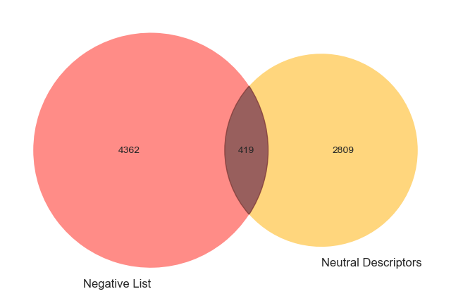
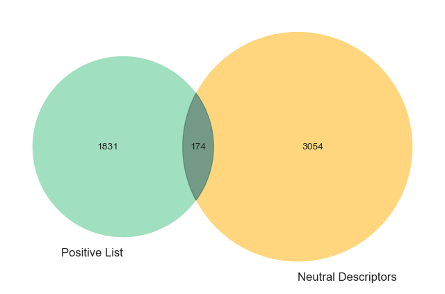
Pre-defined lists of negative and positive adjectives are loaded for comparison with all descriptors currently defined as ‘neutral’ by the textblob classifier.

Plotting these groups on a Venn diagram reveals some overlap, indicating that some tokens may have indeed been inaccurately classified as neutral.

Notably, far more negative descriptors (419) seem to have been potentially misclassified than positive descriptors (174).

# set negative word list
negList=list(pd.read_csv("data/negList.csv")['Negative'])

# create Venn
from matplotlib_venn import venn2, venn2_circles
plt.figure(figsize=(8,8))
v=venn2([set(negList), set(tag_df[tag_df['sentiment']==0]['description'])],
        set_labels = ("Negative List", "Neutral Descriptors"),
        set_colors = ("#FF6F69","#ffcc5c"),
        alpha = 0.8)
v.get_patch_by_id('11').set_color("#7f3734")

# set positive word list
posList=list(pd.read_csv("data/posList.csv")['Positive'])

# create Venn
plt.figure(figsize=(8,8))
v=venn2([set(posList), set(tag_df[tag_df['sentiment']==0]['description'])],
        set_labels = ("Positive List", "Neutral Descriptors"),
        set_colors = ("#88D8B0","#ffcc5c"),
        alpha = 0.8)
v.get_patch_by_id('11').set_color("#518169")

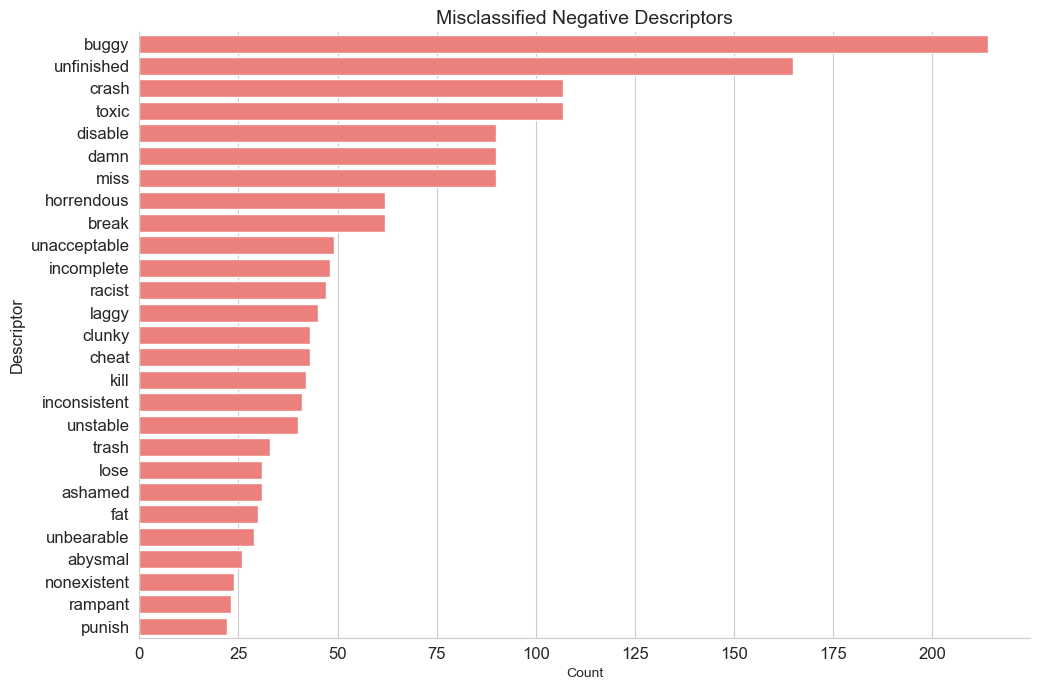
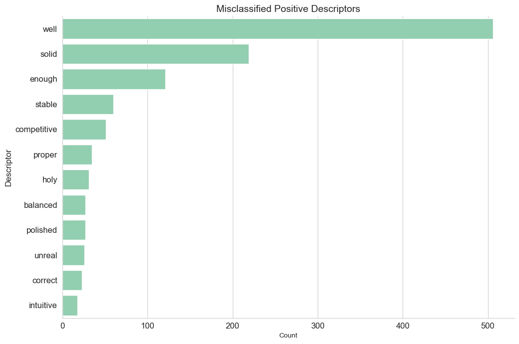
Plotting the highest frequency potentially misclassified descriptors identifies several that should actually be classified with a positive or negative sentiment polarity.

Inaccurate classification is likely due to the absence of these descriptors in the textblob sentiment lexicon. Because of their absence, these tokens are assigned a 0 polarity value and are thus categorised as ‘neutral’.

This can be rectified by modifying the textblob lexicon to include these missing relevant tokens.

# create df of neutral descriptors contained in negative list
# negative list from https://gist.github.com/mkulakowski2/4289441

df1 = tag_df[(tag_df['sentiment']==0) & (tag_df['description'].isin(negList))]
df1 = df1.groupby('description',as_index=False)['aspect'].count().rename(columns={'aspect':'Count'})
# plot negative terms
ax=sns.catplot(data=df1[df1['Count']>=20].sort_values(by='Count',ascending=False),
            kind='bar',
            y="description",
            x='Count',
            palette = ['#FF6F69'],
            height=7,
            aspect = 1.5)
plt.title('Misclassified Negative Descriptors',fontsize=14)
plt.tick_params(labelsize=12)
plt.ylabel('Descriptor',fontsize=12)
plt.tight_layout()
plt.show();

# create df of neutral descriptors contained in positive list
# positive list from https://gist.github.com/mkulakowski2/4289437
df2 = tag_df[(tag_df['sentiment']==0) & (tag_df['description'].isin(posList))]
df2 = df2.groupby('description',as_index=False)['aspect'].count().rename(columns={'aspect':'Count'})

# plot positive terms
ax=sns.catplot(data=df2[df2['Count']>=15].sort_values(by='Count',ascending=False),
            kind='bar',
            y="description",
            x='Count',
            palette = ['#88D8B0'],
            height=7,
            aspect=1.5)
plt.title('Misclassified Positive Descriptors',fontsize=14)
plt.tick_params(labelsize=12)
plt.ylabel('Descriptor',fontsize=12)
plt.tight_layout()
plt.show();